What xwOBA Misses

A better model and the value of speed

A persistent gap between wOBA and xwOBA led me to build a more accurate, better-calibrated model and examine what the remaining residuals reveal about Sprint Speed.

Weighted On Base Average (wOBA) is an advanced baseball metric that measures a player’s total offensive value per plate appearance; the weighting of outcomes (Out,1B,2B,3B,HR) in the metric are a function of their expected run values. Players are also evaluated by their Expected Weighted On Base Average (xwOBA), a model derived estimate of a player’s wOBA on a given PA based on the launch angle, exit velocity etc of their hit. xwOBA is intended to remove things like ``luck’’ from our evaluation of a hitter’s performance. Being an expected statistic, on average we should expect the difference between players wOBA and xwOBA to be 0. Interestingly, when I residualized wOBA by comparing players’ actual wOBA with Statcast’s xwOBA, the gap was not just noise from one year to the next. In fact, there appeared to be a moderate year-over-year correlation at the player level in whether players under- or overperformed their xwOBA. In a residual analysis, a significant amount of this year-over-year stability was explained by players’ Sprint Speed—an intuitive result in which faster players get more out of their balls in play than slower players, controlling for contact quality.

That could mean xwOBA was missing repeatable baseball value. It could also mean my sample was misleading, my calibration was drifting, or I was asking an expected statistic to answer a question it was never designed to answer. Statcast does not provide a great foundation for answering this question, as its xwOBA model is proprietary and only the final number per BIP (ball in play) is accessible by API. This provided a nice two-part opportunity for someone interested in sports analytics: to train, validate, and test my own xwOBA model to try to improve on the performance of Statcast’s model across multiple dimensions, and to use the resulting model to investigate the factors associated with persistent over- or underperformance in MLB.

The result of this project is FAIR xwOBA—Field- and Atmosphere-Informed Realized-contact xwOBA. It predicts the value of a batted ball using contact physics, where it was hit, the park and atmosphere, and the defense’s pre-pitch shape. It does not use the batter’s name, identity, Sprint Speed, age, height, weight, handedness, position, or team. From the outset, I want to be clear that although FAIR xwOBA beats Statcast on core metrics, this is not directly a fair comparison, as my model employs a richer contextual feature set than Statcast claims to use. That said, increased performance is valuable for my aims insofar as, when we residualize wOBA with a better xwOBA model, we can more precisely identify associations between measurable player-level attributes (like Sprint Speed) and their over- or underperformance.

Interestingly, once I residualized wOBA using FAIR xwOBA, the residual Sprint Speed signal became substantially larger, not smaller.

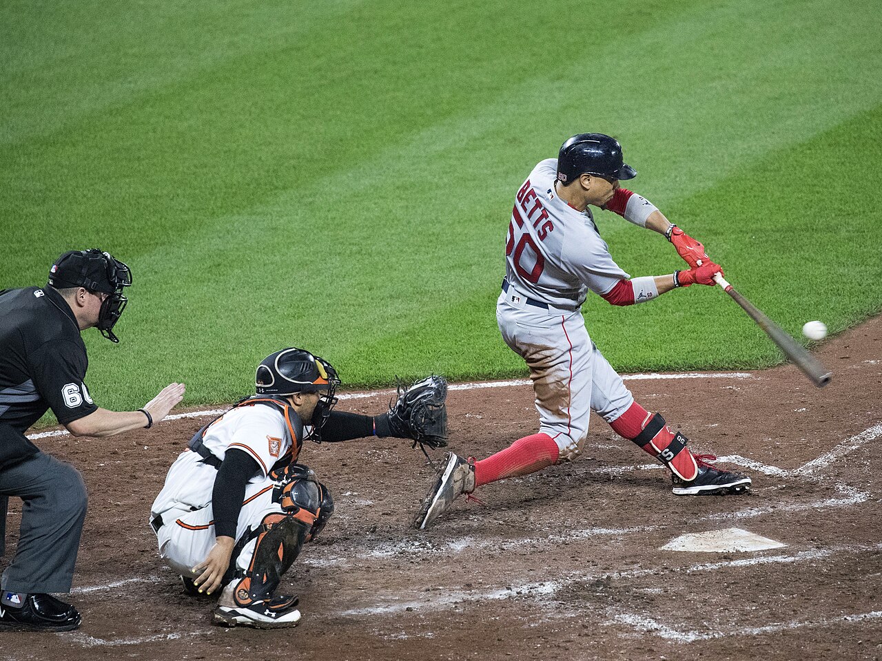
At the moment of contact, the ball tells us a great deal—but perhaps not everything. Photo: Keith Allison, cropped by a Wikimedia Commons contributor, CC BY-SA 2.0.

In this article

• Answer in brief
• What made me think xwOBA was missing something?
• Why didn’t my first rebuild solve it?
• What would a better xwOBA model need to do?
• What is FAIR xwOBA?
• Did it actually beat Statcast?
• Why did the residuals get more persistent?
• What does speed appear to be worth?
• What do two real seasons look like?
• Why not simply put Sprint Speed into FAIR?
• What am I not claiming?
• What did better calibration make visible?

Answer in brief

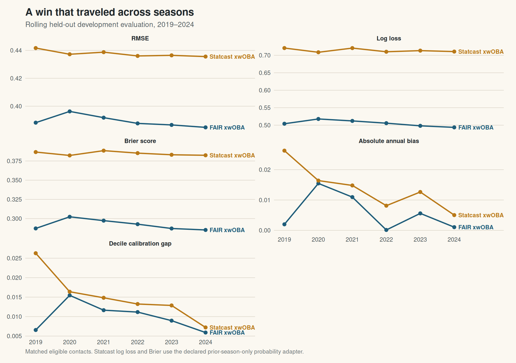
• FAIR beat Statcast on all five reported metrics in every held-out development season from 2019 through 2024: RMSE, five-class log loss, Brier score, annual mean bias, and decile calibration gap.
• After scoring, one Sprint Speed standard deviation was associated with 0.799 run-equivalent units per 100 matched balls in play in FAIR’s residuals.
• On the trait-complete player panel, Sprint Speed, age, height, and weight explain about 51% of FAIR’s measured year-to-year residual persistence.

These are verified rolling development results, not a final untouched-season confirmation. The Sprint Speed analysis is descriptive and post-score.

What made me think xwOBA was missing something?

Expected statistics are useful because they separate a process from its realized result. A line drive caught at the wall and one that lands a foot beyond the glove can come from nearly identical contact, even though the box score treats them very differently. xwOBA tries to replace the realized outcome with an expectation based largely on how hard and at what angle the ball was hit.

My original analysis began at the player-season level. I defined the residual as actual wOBA minus estimated wOBA and then asked whether a player who beat his expectation in one season tended to do it again in the next. Across 1,612 adjacent player-season pairs from 2015 through 2024, the lag-one Pearson correlation was 0.301, with a bootstrap interval from 0.245 to 0.358.

That is at most moderate year-over-year stability, and for the purposes of forecasting individual players, the signal is decidedly weak. That said, it is much too large to describe the residual as pure luck.

The player-trait results made the puzzle more specific. A one-standard-deviation increase in Sprint Speed was associated with a +.0033 wOBA residual in the original model. Using the study’s run-value conversion, that is roughly 0.26 additional run-equivalent units per 100 balls in play—or about one run across 400 balls in play. Height and weight had smaller negative associations, also in intuitively plausible directions. The pattern suggested a simple baseball explanation: a model focused primarily on the batted ball may not fully capture the value created by the runner trying to beat it to first.

Figure 1: The original clue. All 1,612 observed player-season pairs are shown with transparency to preserve the full distribution; the fitted line and annotation report the unweighted Pearson relationship. Sprint Speed had the clearest positive standardized trait association.

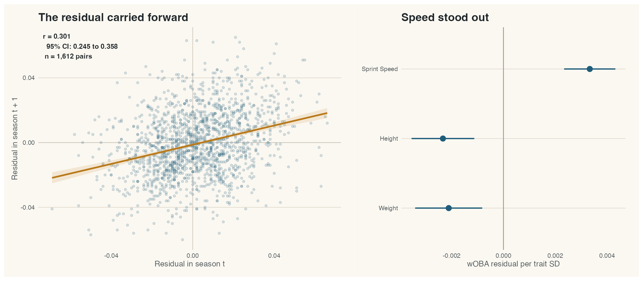
Those estimates came from the original player-season study, not the larger data set I assembled later to train FAIR xwOBA. The observed associations replicated in the larger sample; I merely include the original as part of a reconstruction of the timeline of this project. Getting to FAIR xwOBA was a journey involving a notable but instructive failure to improve on Statcast’s results.

Why and how my first model failed

My first model was built on the instinct that more baseball context would fix the residuals and improve calibration and out-of-sample performance. Add the ballpark. Add whether the park has a roof and whether it was closed that game. Add temperature and field-relative wind. Handle spray direction more carefully. Give the model a physically interpretable proxy for how long the ball stayed in the air. Then throw the richer feature set into a flexible ML model (XGBoost) and see what happens.

The resulting model looked encouraging on average, with lower average bias than Statcast, but its calibration was highly variable from season to season and failed to beat Statcast on calibration overall. Reflecting on the failed model, I saw that I had made a classic error in sports analytics involving models that predict class probabilities but are evaluated on scalar values built from those probabilities: I had optimized a probability model and then treated scalar xwOBA calibration as if it would follow automatically. Naturally, it did not. A model can rank contact well and still run too hot or too cold when the league environment changes. It can improve a pooled score while producing a mean prediction that misses badly in a particular year. I recognized that calibration needed to occur at both the probabilistic level (e.g., whether the predicted probability of a single is close to the observed frequency of a single for a hit with such characteristics) and the scalar xwOBA level (e.g., whether predicted xwOBA values are close on average to the corresponding players’ observed wOBA values).

A richer set of criteria for model evaluation

Based on the previous failures, I settled on three types of evidence with which to evaluate my next xwOBA model.

First, root mean square error, RMSE, asks whether the scalar expected wOBA value is close to the realized value of each contact. Second, log loss and Brier score judge the full five-outcome probability distribution. A model should not receive the same credit for assigning a single and a home run equal probability just because their average happens to land near the right scalar value. Consider a batter who hits a double, and assume that a model assigned high and approximately equal probabilities to a home run and a single, and almost no probability to the double outcome. The resulting scalar xwOBA would be very close to the observed outcome because the single and home-run values average to approximately the value of a double (so RMSE would be low), but the probabilistic calibration would be atrocious (log loss and Brier score would be high). This example illustrates how one type of calibration does not follow from the other. Both types matter because scalar calibration determines whether xwOBA is trustworthy as an estimate of contact value, while probabilistic calibration determines whether the model is correctly describing how that value is likely to be realized—and a useful expected statistic should do both. The third and final type of evidence, annual bias and decile calibration gaps, asks whether predictions remain trustworthy across seasons and across low-to-high expectation groups. Ideally, the model should be able to capture season-level changes that affect outcomes, such as an evolving baseball rules landscape.

Lower is better for all five numbers. The important constraint is temporal: every score must come from a season the model had not seen when it was trained or calibrated. This is key, as the flexibility of advanced ML models is a double-edged sword: it allows us to capture nonlinear and interaction effects, but at the risk of overfitting to the training sample, which tends to result in unsatisfactory out-of-sample performance on new data.

For each held-out development season from 2019 through 2024, I reconstructed the information that would have been available before that season began. To evaluate season (y), the XGBoost learner was trained only on seasons through (y-2). Games from season (y-1) were then divided into separate whole-game groups for hyperparameter tuning and probability calibration. Keeping entire games together prevented contacts from the same game—and therefore the same pitchers, hitters, weather conditions, and defensive context—from appearing on both sides of a development split.

The scalar xwOBA calibration layer was also estimated without using outcomes from season (y). It relied on out-of-fold predictions from seasons that had already been completed, so every residual used to learn the correction came from a prediction made without access to that observation’s outcome. The small ground-ball adjustment followed the same rule: it could learn only from previously completed seasons and could not update itself using the season it was about to score. The ground-ball correction is a deliberately narrow, history-only adjustment that accounts for a recurring out-versus-single error on weakly hit ground balls without introducing player identity or traits into FAIR, a model feature I adopted from Statcast.

Each annual evaluation therefore functioned like a historical deployment exercise. The model, probability calibrator, scalar calibrator, and ground-ball correction were all fixed using information available before Opening Day; only then was the next season revealed and scored. At no point could an outcome from the held-out season influence its own prediction, directly or indirectly.

That chronology matters more to me than squeezing another decimal point from a random train/test split. Baseball changes. The ball changes. Defensive rules change. A model that cannot carry its expectation forward is not well calibrated in any sense that matters.

What is FAIR xwOBA?

FAIR stands for Field- and Atmosphere-Informed Realized-contact xwOBA. “Realized-contact” is deliberate. This is not a claim to have isolated a context-free essence of contact quality. FAIR estimates what a batted ball was worth in the park, weather, roof state, rule era, and pre-pitch defensive context in which it occurred.

ContactLaunch speed, launch angle, spray coordinates, and a ballistic hang-time proxy

EnvironmentCanonical park, temperature, field-relative wind, roof status, and shift-rule era

DefensePre-pitch infield and outfield alignment categories—not fielder identity or outcomes after contact

BackboneA regularized five-class XGBoost model for out, single, double, triple, and home run

CalibrationPrior-season temperature scaling followed by prior out-of-fold scalar calibration

Local correctionA small prior-only generalized additive model (GAM) adjustment to the out-versus-single margin on selected negative-angle ground contact

In plain terms, the primary XGBoost model first predicts the probability of each outcome (out, 1B, 2B, 3B, HR) based on the contact, environment, and defensive features described above, with the constraint that the probabilities sum to one. The five class probabilities are then multiplied by their associated numeric wOBA values and summed, resulting in one xwOBA value per BIP. FAIR then applies a separate monotone scalar calibration layer built using a GAM. Keeping the stages distinct is important: temperature scaling protects the probability distribution, while the scalar layer corrects the expected wOBA scale that readers actually use. This explains why we split each calibration set into two disjoint subsets: it allows us to calibrate both aspects using independent data.

Sprint Speed is not an input. Neither are player names, IDs, age, body size, handedness, position, team, or fielder identity. Those fields are joined only after predictions have been written and hashed. This is intentional: by excluding these features from the model, we can go on to residualize wOBA with FAIR xwOBA and then estimate associations between these measurable player attributes and year-over-year wOBA under- and overperformance.

There is one wrinkle in my “player-free” description of FAIR’s feature set. Defensive alignment is game context, not a declared player trait, but defenses choose alignments in response to what they know about hitters. FAIR therefore has no player identity at scoring time while still receiving a contextual variable that can indirectly encode prior hitter tendencies. During baseball’s defensive-shift era (thankfully a short era), I expect that this confounding was notable. That makes the realized-contact description more honest than calling the model purely intrinsic.

Did FAIR xwOBA beat Statcast?

Because FAIR xwOBA uses a richer set of inputs than Statcast’s public documentation indicates—although its proprietary specification is not fully known—the comparison is not strictly like-for-like. Across the six rolling held-out seasons, FAIR’s advantage was not confined to a single metric or a convenient year. It had lower RMSE, log loss, Brier score, absolute annual bias, and mean absolute decile gap in every season.

Figure 2: FAIR was lower on every metric in every held-out development season. Each panel has its own vertical scale; lower is better throughout.

The equal-season averages put the size of the result in context. FAIR’s RMSE was 0.3892, versus 0.4376 for Statcast. Log loss was 0.5053 versus 0.7140; Brier score was 0.2920 versus 0.3846. FAIR’s average absolute annual bias was 0.0059, less than half Statcast’s 0.0139, and its mean absolute decile gap was 0.0099 versus 0.0151.

What the probability comparison means. Baseball Savant publishes scalar xwOBA but not the five outcome-class probabilities needed for log loss or Brier score. RMSE, bias, and decile calibration use public Statcast xwOBA directly. Log loss and Brier use a separately declared probability adapter trained only on prior seasons. The Methods page defines both comparators.

This is strong development evidence, but it is not a final untouched test. The exact FAIR candidate never opened 2025 or partial 2026. The broader project had already looked at 2025 when I first analyzed the persistence of players’ over- or underperformance, so I do not treat it as pristine confirmatory evidence. The completed future-season test remains the harder standard.

Why did the residuals get more persistent?

In the introduction, I mentioned that residualized wOBA became more stable year over year using FAIR, despite FAIR being a better-calibrated and more accurate model. Limiting my sample to players with at least 100 BIPs, FAIR’s centered weighted year-to-year residual correlation was 0.270, compared with 0.190 for Statcast. From one perspective, lower persistence was supposed to mean a more player-neutral model. FAIR was better on every prediction metric and worse on that diagnostic.

Accordingly, one interpretation is that FAIR still has a systematic defect. Another is that, after removing more contact and environmental noise, its residuals contain a higher proportion of repeatable player-specific value that the model intentionally cannot see. This links back to my second goal for the project: quantifying the association between player attributes like Sprint Speed and observed performance, controlling for contact quality, defensive alignment, environmental conditions, et cetera.

The trait decomposition supports the second interpretation—partially. On the complete-case panel, Sprint Speed alone reduced FAIR’s measured persistence by 41.8%. Sprint Speed, age, height, and weight together reduced it by 51.3%. For Statcast, the corresponding reductions were 11.0% and 21.5%.

Figure 3: Measured traits explain much more of FAIR’s repeatable residual structure than Statcast’s. These are descriptive reductions on the shared trait-complete panel, not additive causal shares.

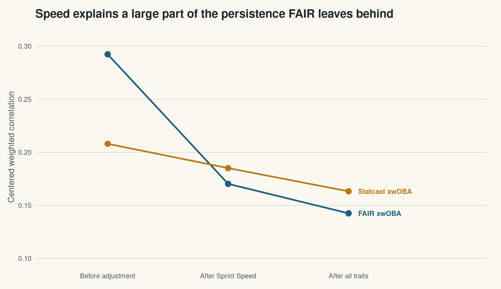
“Explains” here means that the correlation falls after residualizing player-season errors on those measured attributes. It does not mean that half the residual is caused by those traits, nor that the traits are measured without error. But it makes random year-to-year luck an inadequate explanation for the whole pattern.

The result also changed how I think about neutrality. Prediction neutrality is a design property: FAIR cannot look up who the batter is or use a stored physical trait. Residual neutrality is an empirical property: after scoring, do identifiable player characteristics still organize the errors? A model can satisfy the first and fail the second because baseball players possess real, repeatable skills that were intentionally withheld. This poses an interesting question—bracketing causal concerns, what is the value of speed in baseball? What do notable speedster Corbin Carroll’s legs bring to the Diamondbacks’ offense alongside his bat?

The apparent value of speed

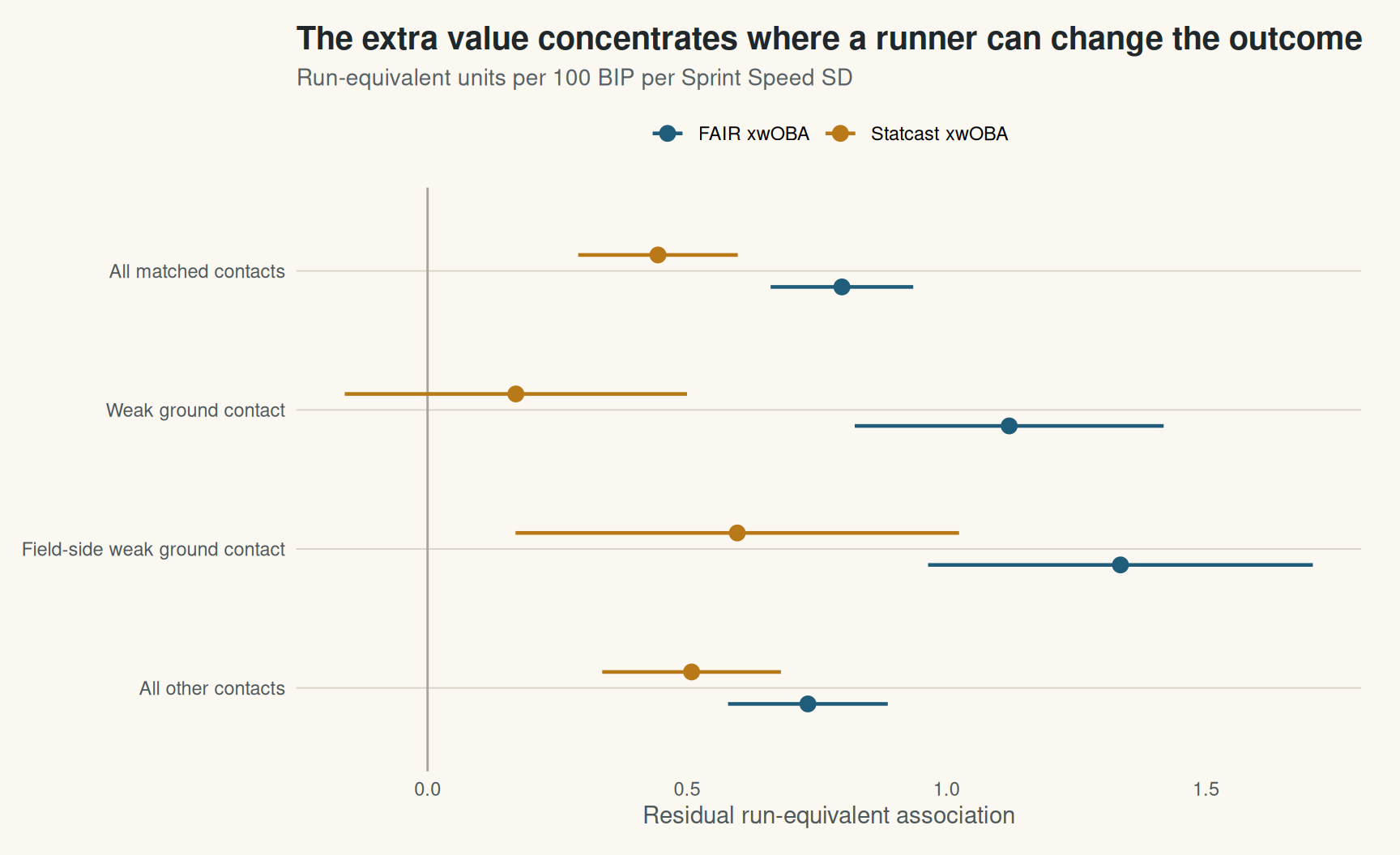
On the matched player-season panel, one Sprint Speed standard deviation—1.39 feet per second—was associated with 0.799 run-equivalent units per 100 balls in play in FAIR’s residuals. The whole-player bootstrap confidence interval ran from 0.661 to 0.941. Statcast’s corresponding association was 0.444.

The location of the signal is revealing. It is strongest on weak ground contact, especially when the ball is hit toward a field side rather than directly up the middle. I determined this by estimating the Sprint Speed–residual association separately within predefined contact regions and comparing the coefficients and uncertainty intervals. The result is intuitive because weak grounders create the closest races between batter and throw, while balls hit toward a field side often require a fielder to move laterally and complete a longer, less direct play at first.

Figure 4: The Sprint Speed association is largest on weak ground contact, especially toward a field side. Intervals are player-clustered descriptive 95% intervals.

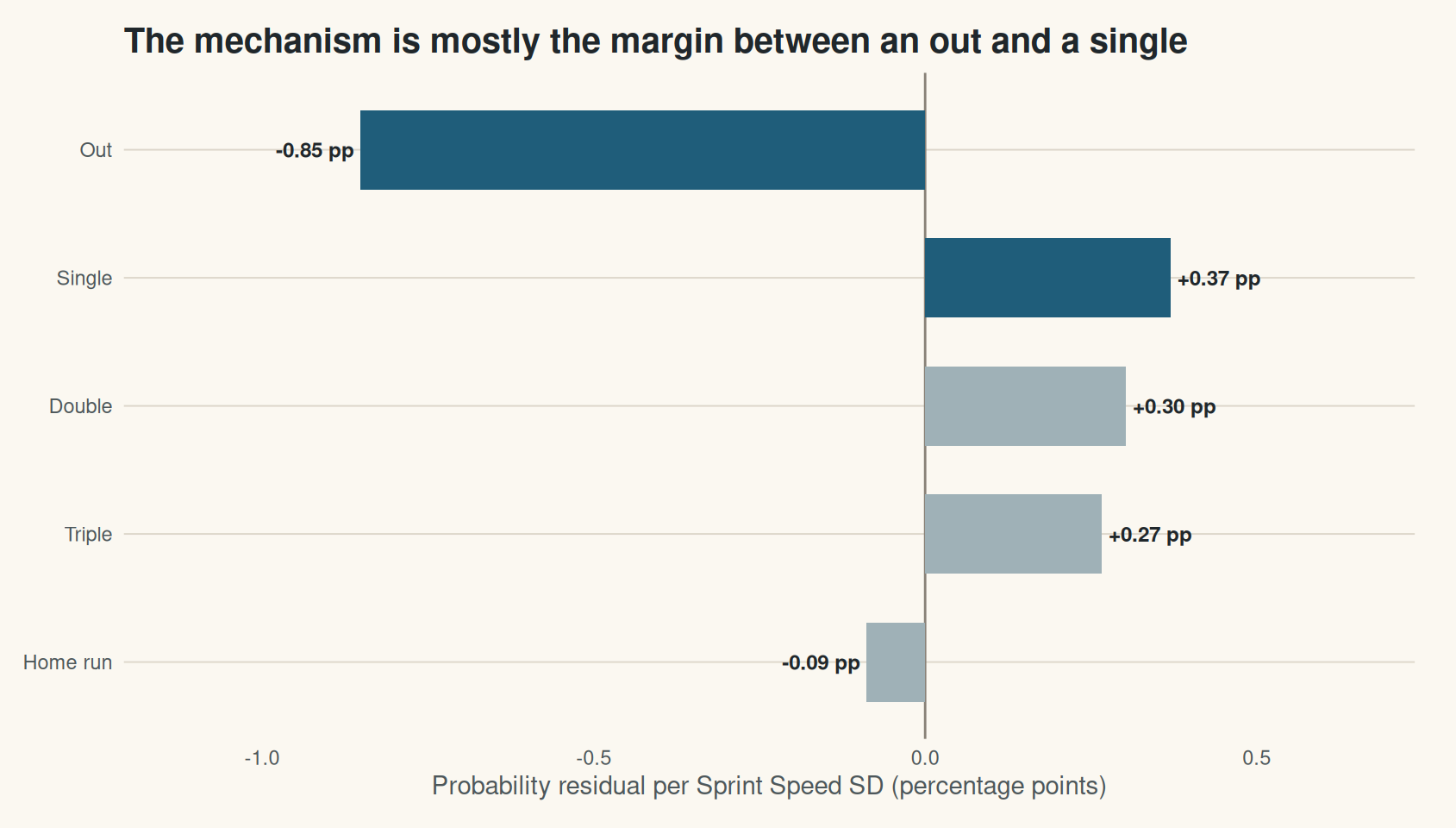
The class-probability residuals tell the same story from another angle. With each Sprint Speed SD, FAIR overpredicted outs by 0.852 percentage points and underpredicted singles by 0.370 points. The single-minus-out residual margin changed by 1.222 percentage points. That is exactly where a fast runner should matter most: not by turning a routine fly ball into a home run, but by shifting borderline ground contact from an out toward a single.

Figure 5: FAIR’s Sprint Speed residual signal is led by fewer outs and more singles than its player-free probabilities expect. Values are outcome-probability residual percentage points per Sprint Speed SD.

For a more intuitive scale, consider comparing a very slow player with a very fast player. The 10th-to-90th percentile Sprint Speed gap in this sample is 3.5 feet per second, or about 2.51 standard deviations. Across 400 balls in play—the neighborhood of a full season’s contact—that difference corresponds to approximately eight run-equivalent units in the population regression.

That is not an estimate of stolen-base value. It is not WAR. It is not RE24 or full-plate-appearance batting runs. It is a season-specific wRAA-style translation of contact-only residuals, conditional on the measured traits in the model. But it is far too large to dismiss as leftover noise.

An illustrative example

The population coefficient is the headline result; individual seasons help make its scale tangible. A (quasi-cherry-picked) comparison between two actual player-seasons is both fun and illustrative. I did want my example to be selected in a somewhat principled manner, so I fixed the example rule before displaying names: I filtered to players with at least 350 matched contacts, took the top and bottom Sprint Speed deciles, and then selected the most positive fast residual and the most negative slow residual. That rule selects Corbin Carroll’s 2023 season and Miguel Cabrera’s 2021 season.

Fast runner illustration

Corbin Carroll

2023 season

+0.070

actual contact wOBA minus FAIR xwOBA

Matched contacts

432

Sprint Speed

30.1 ft/s

Speed percentile

99th

Total run-equivalent residual

+25.3

Slow runner illustration

Miguel Cabrera

2021 season

-0.068

actual contact wOBA minus FAIR xwOBA

Matched contacts

350

Sprint Speed

24.0 ft/s

Speed percentile

2th

Total run-equivalent residual

-19.7

The cards do not say Carroll created 25 run-equivalent units with his speed or Cabrera lost 20 because of his. Those totals translate each season’s entire FAIR residual, which also contains defense, measurement error, unmeasured skills, and ordinary variation. Their purpose is narrower: show what the fixed-rule extremes behind the population relationship look like without turning the release into a player leaderboard.

What am I not claiming

I tried to be careful throughout this write-up about what I claim the project shows, but it is worth giving this a little more time.

Five limits matter. These are rolling 2019–2024 development results, not the final untouched-season test. The Sprint Speed estimates are descriptive associations, not causal effects. The sample contains matched eligible batted-ball contacts rather than complete plate appearances. Pre-pitch alignment may indirectly encode how defenses respond to known hitters. And Statcast log loss and Brier require a declared prior-season probability adapter because Baseball Savant does not publish the underlying five-class probabilities.

There is another conceptual limit worth keeping in mind. A more accurate expected-value model is not guaranteed to have less persistent player-level residuals. If it removes environmental and contact noise more effectively, the repeatable value intentionally excluded from its inputs can become easier to see. Persistence can be evidence of a model defect, evidence of omitted skill, or some combination of both. The trait and mechanism analyses help distinguish those stories; they do not settle them permanently.

What did better calibration make visible?

I began with a residual that looked too persistent to be luck. The first modeling pass taught me that better average prediction was not enough: the expectation also had to remain calibrated when time moved forward. FAIR’s rolling results suggest that contact physics, environment, defensive context, and explicit calibration can improve RMSE, probability loss, and calibration at the same time.

But the project became more interesting after that success. FAIR did not erase player structure from the residual. It clarified it. Faster players beat its player-free expectation in a repeatable and mechanically plausible place: the boundary between a ground-ball out and a single. Measured traits explain about half of the persistence the model leaves behind, and the 10th-to-90th percentile speed contrast corresponds to roughly eight run-equivalent units across a full season’s worth of balls in play.

That number is not a new WAR component and should not be treated like one. It is a conditional descriptive estimate from a deliberately limited contact model. Still, it changes the original question. The remaining residual is not merely an embarrassment for xwOBA to eliminate. It can also be a measurement instrument.

Sometimes the most useful thing about a better expected statistic is not just that it predicts the result more accurately. It is that, once the expectation is trustworthy, what remains becomes worth studying.

Continue to the full methods or audit and reproduce the public evidence.